
Research
What is Finsler geometry?
A. Motion of objects and the minimum distance
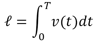
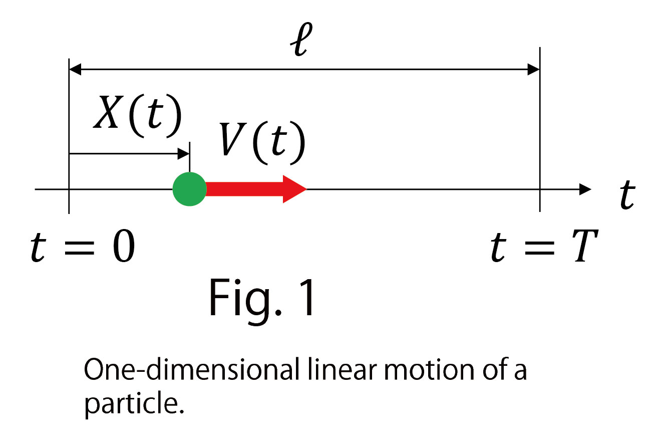
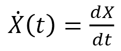
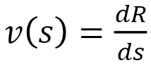
Objects linearly move without a force acting on them (Fig. 1). In this linear motion, the distance  is determined by velocity
  and time
  . Thus, we have distance = velocity × time. In general, is given by the integral
Moreover, the distance can be written as an integral on the real number line such that
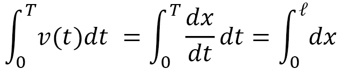
by using 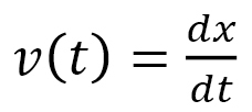 Let us look at this expression as a formula for the motion distance. We feel that the individuality of the motion-like velocity is disappearing. Thus, from the fact that is the distance between P and Q on the 2-dimensional plane, for example, we have the following rule
- Any object linearly moves with a constant velocity if there is no force acting on it
- Its distance is the minimum distance between the two points
(A-1)
However, is (A-1) always true?
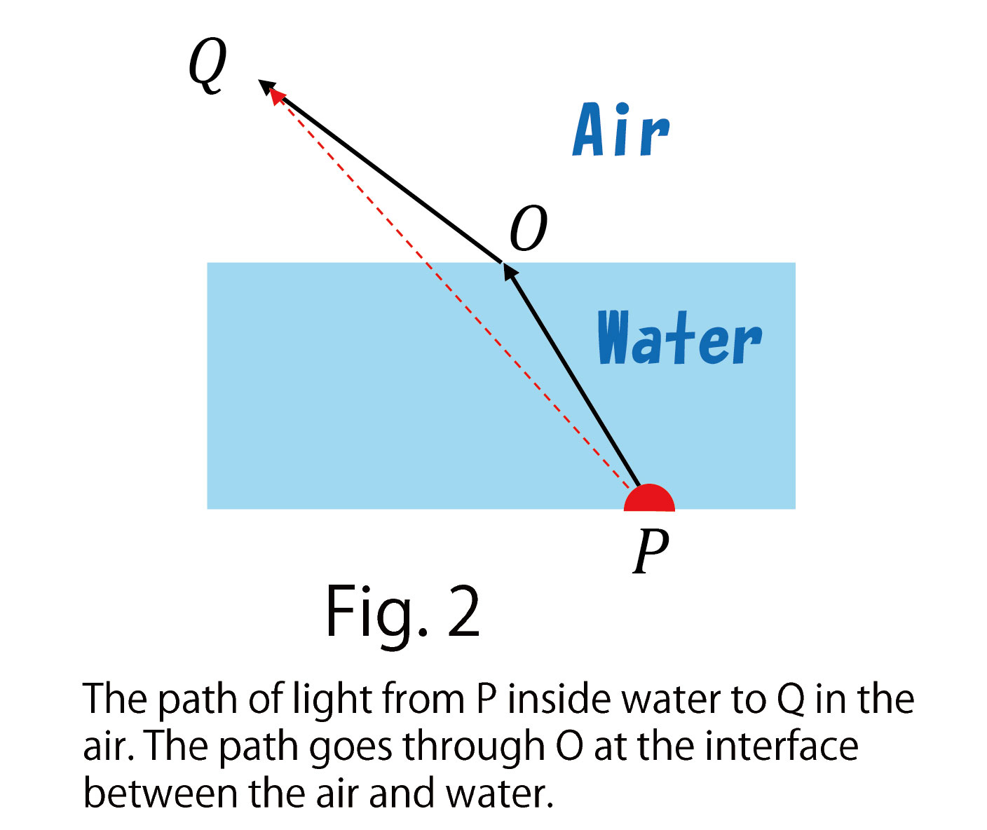
Let us consider the case in which light goes from inside water to the air by regarding the light as an object (Fig. 2).
Light does not go along the straight line from P to Q, as it follows the well-known refraction phenomenon.
The reason is that the velocity of light in the water is slower than that in the air.
Indeed, the light moves from P to Q with the minimum time, and hence, the light refracts.
It is also possible to consider that rule (A-1) cannot explain the refraction attributes to the disregarding of velocity, which are an individuality of motion.
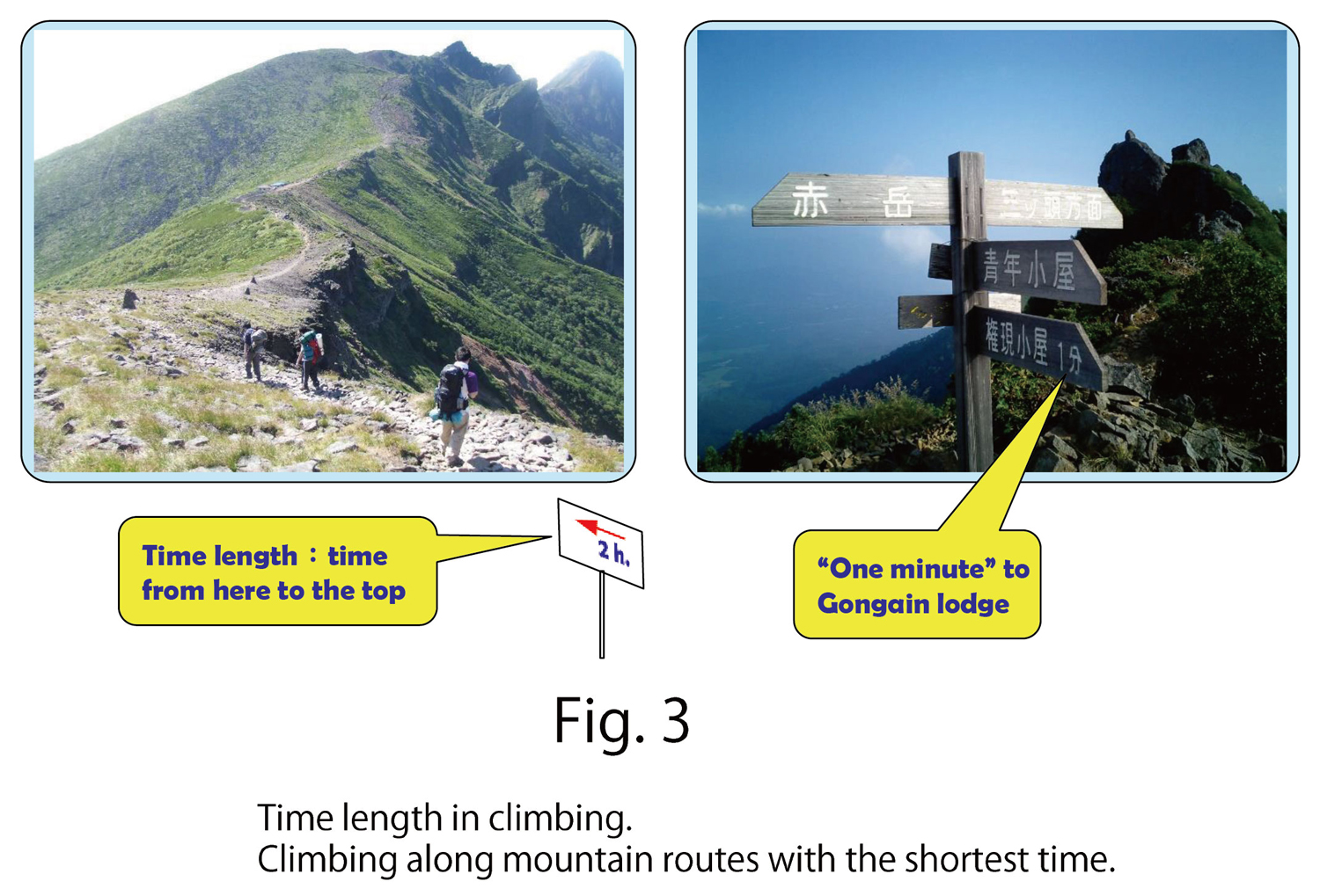
For another example, let us consider mountain climbing (Fig. 3).In this case, the climber is an object, and their walking speed is .
From base to top, the optimal climbing route is not always of the minimum distance. Instead, it is a path that connects the base and top with the minimum time. Many climbing routes are winding and go along ridges, as shown in Fig. 3, and the path lengths are not the minimum length.
On mountains, any distance is presented as a time, such as “2 hours from here to the top”. Indeed, the most critical fact for climbers is how long it takes from here to a lodge on the top or how long it takes to get there and come back. Time distance governs mountain climbing.
Moreover, in climbing, times for going and returning are different, such as 2 hours to go and 1 hour to return. This difference comes from the fact that the walking speed for going is different from that for returning.
In this way, by using the time distance, which is different from the ordinary distance, we expect that rule (A-1) can be applied to light refractions and climbing mountains without modification. However, to establish a correct formulation of time distance, it must be defined mathematically. This was done by Finsler (Ref. [1]),
B. Time distance in Object Motion
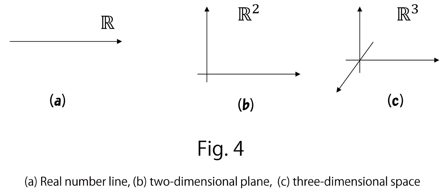
Let us consider the ordinary distance first before going on to the time distance introduced by Finsler. Since numbers describe the position and velocity in practice problems in physics, we mathematically use the distance in the real number. The plane is made of two real number lines, and the three-dimensional space is made of three real number lines (Fig. 4). In physics,
distance is defined by assuming that the distance that light moves in a second in a vacuum is 1. Moreover, units are specified in physics in a slightly complex manner. However, by assuming the distance 1[m] as the real number 1, we can study any motion on the real number line.
- Ref. [1]: Makoto Matsumoto, Keiryou Bibun Kikagaku (in Japanese), Shokabou, 1975.
Now, what is the time distance introduced by Finsler?
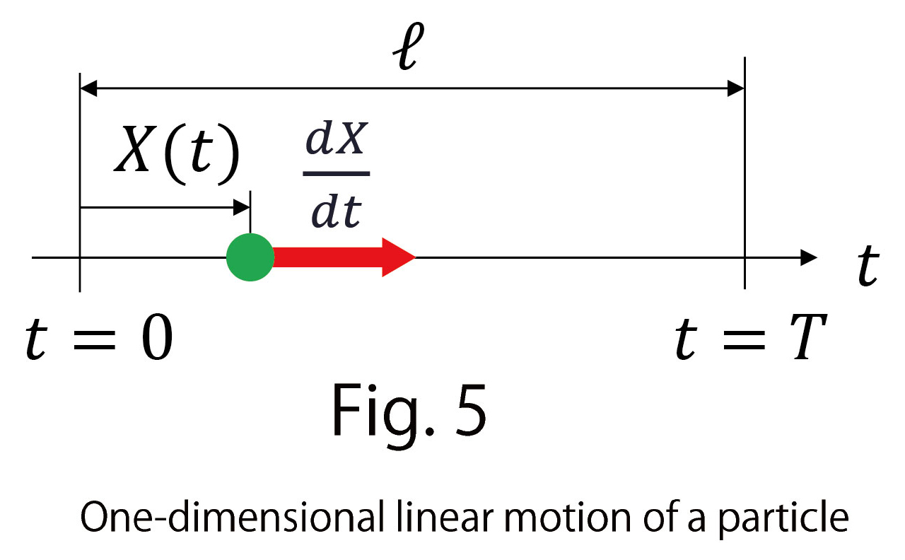
Here, within my understanding, I will explain it by modifying the contents written in Ref. [1] to the linear motion of objects. Let  ,
,  ,
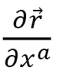
,  be the time, position, and velocity of a particle, and be the distance between the positions at
  and
and  (Fig. 5).
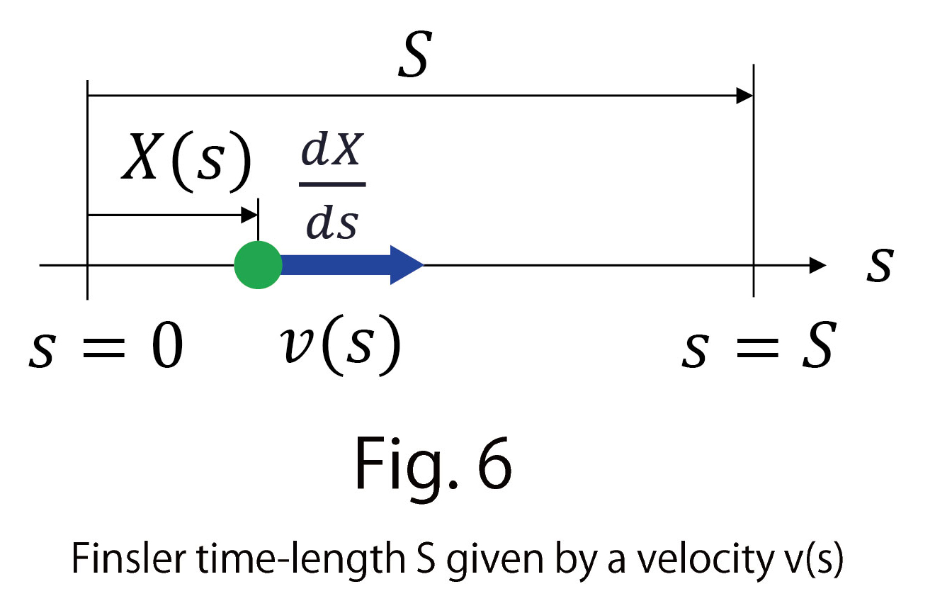
In addition, we assume another motion along the same direction of  with velocity
  , which is not always identical with (Fig. 6). In this case, we define parameter
  , instead of , satisfying
(B-1)
Here, and are assumed to be functions to each other like a transformation of time units. This parameter is defined such that the velocity  with respect to is identical to the given velocity , and it is called “time distance of Finsler.” can also be obtained with the so-called Finsler function, which is a function of position and velocity,
(B-2)
such that
(B-3)
Indeed, we have
(B-4)
which can be used for the definition of the time length .  is independent of any replacement of the integration variable. From this, is a length that is different from the standard length
  (Fig. 5). If
  , then we have
 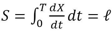 , which is the standard length. If
 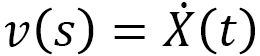 , we have
 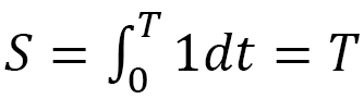 , which is the time, and therefore, we can call the general time length.
An important property is that the time distance depends on the direction. This dependence comes from the fact that can be given to be dependent on the direction. For his reason, the distance shown in Fig. 6 is written by the arrow in the same direction with . In the opposite direction, is defined by another, different from that in Fig. 6. This property is not shared with the standard length in Fig.5 and can be applied in anisotropic deformations.
C. Application of Time Length to Materials Science
Here, we try to apply the time length to the anisotropic deformation of materials by utilizing the direction dependence (time difference between go and return) (Ref. [2]).
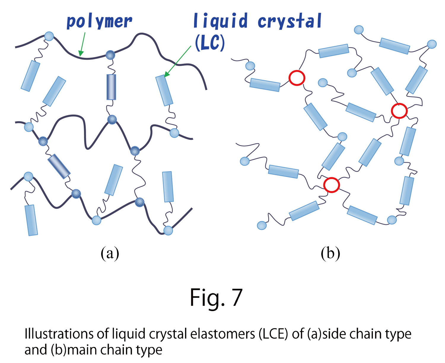
C-1. Anisotropic Deformation of Liquid Crystal Elastomers (Refs. [3, 4])
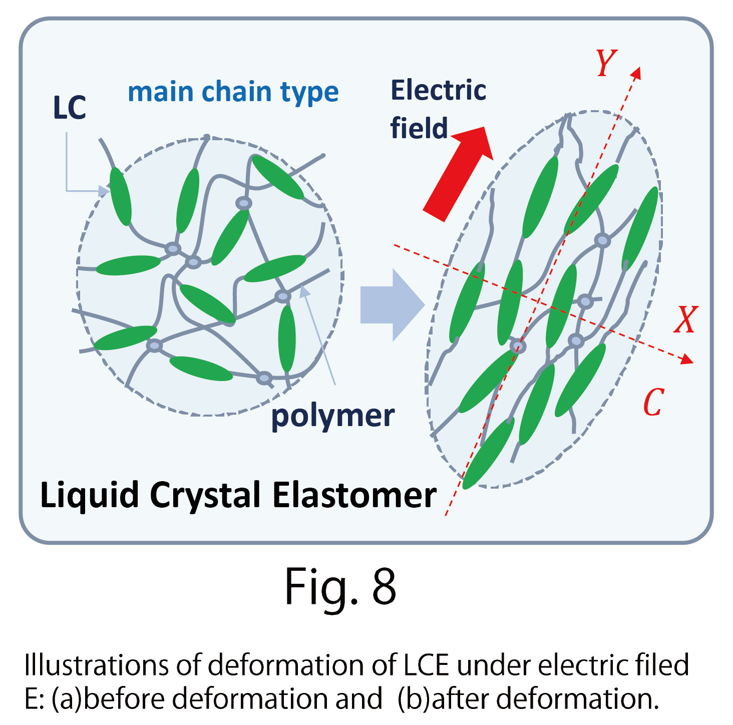
As an example of anisotropic deformations, we consider the so-called liquid crystal elastomer (LCE), composed of chemically bonded polymers and liquid crystal molecules (Fig. 7). LCE deforms oblong in the direction of the applied electric field and shrinks to its perpendicular direction (Fig. 8).
The problem is why such deformation occurs. Many studies, such as first-principle simulations, have been conducted in regard to this problem. Our study, introduced here, is one of them.
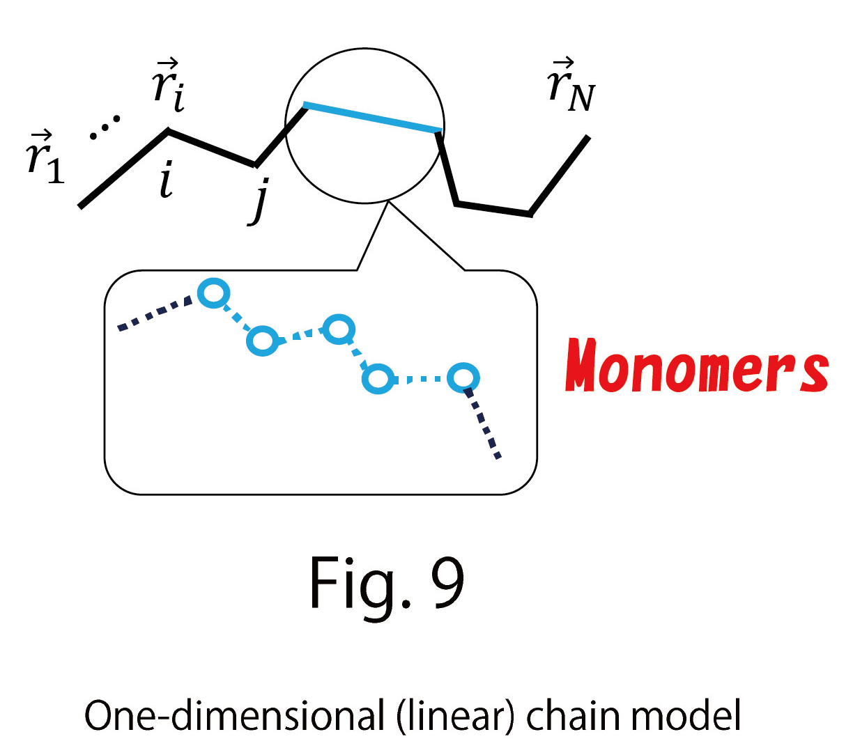
If we focus on the polymer, its Hamiltonian for tensile energy is given by the sum of the length squares  between monomers such that
(C-1)
where  is the position vector of the monomer
  , and
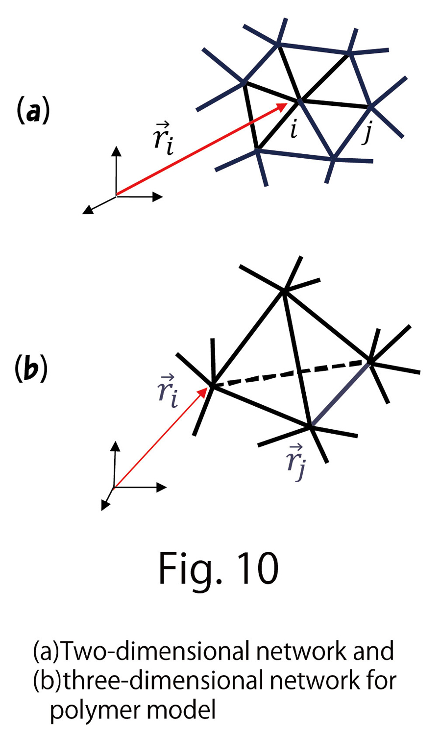
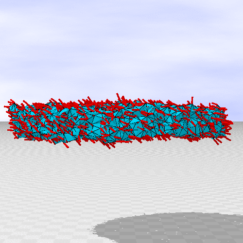
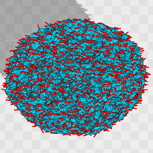
, and  denotes two neighboring monomers(Fig. 9). A model in which this type of Hamiltonian is assumed in the case of one dimension is called a linear chain model in polymer physics. Here, we extend this linear chain model for LCE to two-dimensional networks and further to three-dimensional networks (Fig. 10).
 in Eq. (C-1) can be written as a three-dimensional integration of the local coordinates
  such that
(C-2)
We should note that in Eq. (C-1) has no property to deform into some specific direction. For this reason, in Eq. (C-1) is an isotropic Hamiltonian. To implement the deformation anisotropy, we should include an anisotropy stemming from LC molecules in this Hamiltonian.
- Ref. [2]: H.Koibuchi, H. Sekino, Physica A 393, pp.37-50 (2014) https://doi.org/10.1016/j.physa.2013.08.006
- Ref. [3]: E.Proutorov, H.Koibuchi, J. Phys. (Cond.mat.)30,405101(2018) https://doi.org/10.1088/1361-648X/aadcba
- Ref. [4]: K. Osari, H.Koibuchi, Polymer,114, pp.355-369(2017) https://doi.org/10.1016/j.polymer.2017.02.065
For this purpose, we introduce one-dimensional energy
(C-3)
which is obtained by imposing the 3-dimensional energy (C-1) on line C along the X-axis (dashed line) in Fig. 8. The C-axis is assumed to be parallel to the X-axis for simplicity. Let  be a local coordinate of line C, then the sum
  can also be written as
(C-4)
and the derivative is given by
(C-5)
The reason for introducing  is that the molecular positions move only slightly, unlike the case of particle motion. Therefore, we consider a state function on the C-axis instead of the position
  for a particle. Since the function is defined by a line integral of one-dimensional elastic energy, it increases with increasing like the position . Thus, we have a correspondence
| phenomenon | coordinate function | origin of anisotropy | definition of Finsler length | anisotropy |
|---|---|---|---|---|
| particle motion | |
direction dependent velocity |
 |
direction dependence of |
| Liquid Crystal Elstomer | |
direction of internal condition |
 |
direction dependence of |
We call the coordinate function because determines the time length of Finsler.
From this correspondence, we obtain a 3-dimensional anisotropic Hamiltonian if the following conditions are satisfied:
- Anisotropy stemming from directions of LC molecule is successfully implemented in one-dimensional elastic energy
- Time length of Finsler and the metric functions are obtained by the anisotropic energy
- The same procedures can be performed in the other two directions
For this purpose, we define the Finsler function by using the functions  and
and such that (Fig. 11(a))
(C-6)
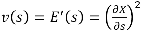
Figure 11(a) is an enlarged illustration of the C-axis in Fig. 8. The problem is .
We find from Fig. 11(a) that the angle  between the LC direction
  and the C-axis is large
 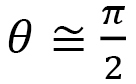 for polymer configurations vertical to the C-axis. In contrast, is small
 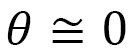 for polymers parallel to the C-axis. Thus, we define by
(C-7)
where  is a small positive number
  If is large
  becomes constant, the time distance defined by
 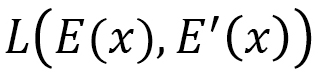 is the standard distance, and no anisotropy is expected. In this sense, we consider to be a strength parameter of anisotropy.
The next problem is: How do we obtain the anisotropic tensile energy from the Finsler function . For this purpose, we calculate the metric function g from by using the formula
(C-8)
where  implies that
  is element (1,1) of the 3x3 matrix g. This means that is the element corresponding to the
  axis in the local coordinate shown in Fig. 12(a). By using
  axis in the local coordinate shown in Fig. 12(a). By using
  ,
,  is defined by
(C-9)
and the Finsler metric is given by
(C-10)
 is the inverse and
  is the determinant. If this Finsler metric is inserted to the Hamiltonian described by a curvilinear coordinate
(C-11)
then anisotropy originating from the direction of LC molecules can be implemented. Here, we omit the details, however, by discretizing Eq. (C-11) on tetrahedrons in Fig. 12(a), we have
(C-12)
where  、
、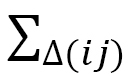 denotes the sum over bonds ij and the sum over tetrahedrons
  sharing the bond ij, and
  is defined as the bond ij of tetrahedron ijkl in Fig. 12(b). This can also be written by using
  the sum over tetrahedrons and
  the sum over bonds ij of the tetrahedron such that
(C-13)
Now, the problem is whether the expected anisotropy is obtained for materials deformation if the Finsler metric is used. The expected anisotropy can be qualitatively understood as follows:
For 
From the one-dimensional energy 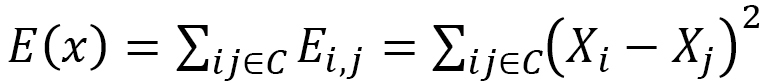 and
and  we obtain
(C-14)
on the C-axis in Fig. 11(a).By integrating this, we also have
(C-15)
where is assumed to be a small number. Since the left-had side of Eq. (C-15) is 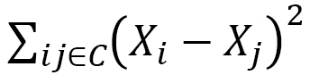 , we obtain
(C-16)
This expression implies that the distance between monomers along the axis perpendicular to the electric field becomes small.
Moreover, by considering that the elastic energy includes a tension coefficient  in general and that such elastic energy becomes constant, we find from Eq. (C-16) that the effective tension coefficient along the C-axis becomes large. In other words, the origin for anisotropic deformation of LCE under electric field is that the coupling constant between molecules dynamically changes. Rather, it seems correct that the coupling constant dynamically changes.
For :
This is the case when viewing the same configuration from the Y-axis. From the same argument above, we find that  , This implies that LCE deforms oblong along the direction of the electric field.
C-2. Response of Liquid Crystal Elastomer (LCE) under an Electric field (Ref. [3,4])
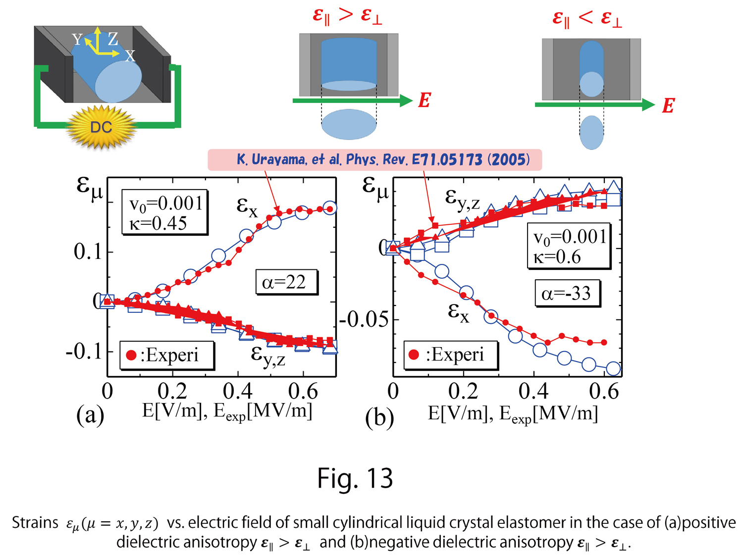
Here, we present some of the simulation results on the response under an electric field. Figure 13 shows the simulation results strains  vs. electric field in Ref. [3] together with experimentally observed results reported in Ref. [5], where the electric field is applied on a small cylinder, and strains in the three directions are measured. Figure 13 (a) show the data in the case of positive dielectric anisotropy
  , and Fig. 13 (b) show the data for negative dielectric anisotropy
  , Detailed information on the assumed parameters is omitted here; however, we find that the simulation results are in good agreement with the experimental data.
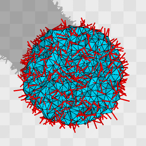
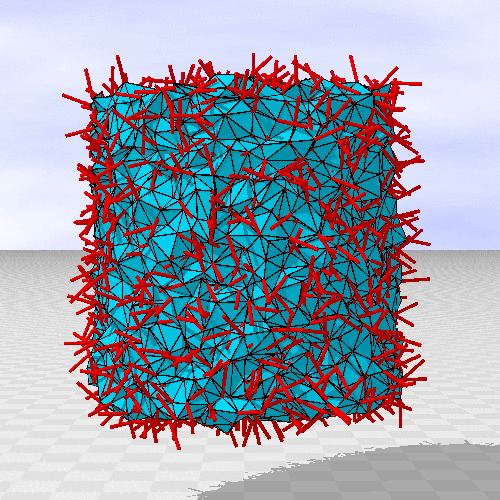
Figure 14 shows animations for positive of positive dielectric anisotropy. The strain is larger than an actual one to make the deformation clear. We find that the direction of LC molecules (small red cylinders) aligns along the electric field direction, which accompanies the shape deformation.
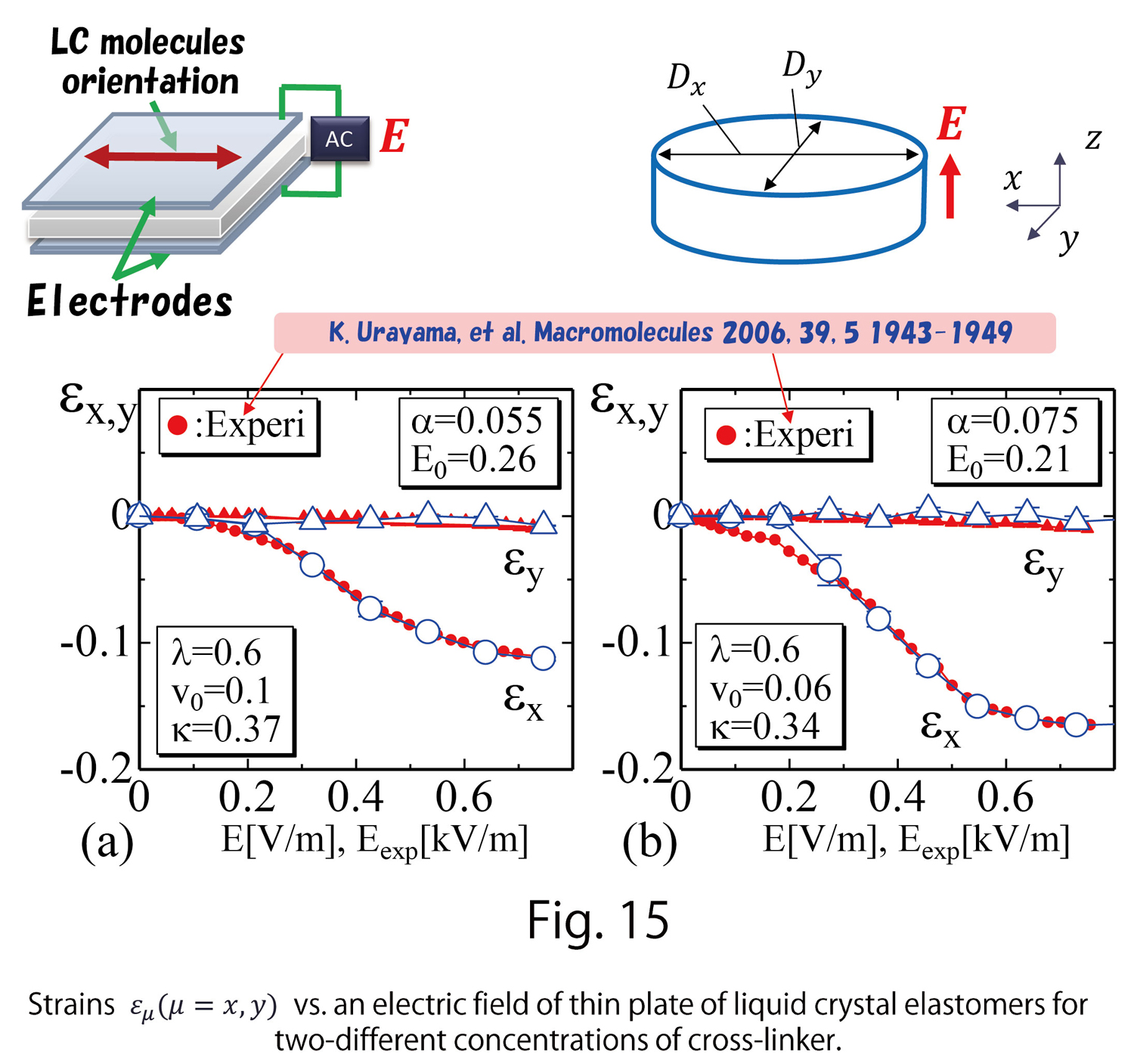
Figures 15(a),(b) show the simulation results in Ref. [3] together with experimentally observed data reported in Ref. [6], where strains  of a thin LCE plate are measured. In this thin plate, the LC molecules align along the direction (x-axis) indicated in Fig. 15 at the beginning. Then, the LC direction change from the x-axis to the z-axis for increasing electric field applied to the z-direction. Therefore, no deformation is expected in the y-direction because no change is made in the LC direction along the y-axis. A thickness change is expected in the z-direction, However, the x-axis is the major change direction. The simulation results demonstrate these experimentally observed facts well.
Figure 16 is an animation showing the deformation of LCE. In this case, the strain is larger than the experimentally observed one. We find that the plate clearly does not deform into the y direction.
- Ref. [5] K. Urayama, et al. Electrically driven deformations of nematic gels, Phys. Rev. E71, 05173 (2005)
- Ref. [6] K. Urayama, et al. Deformation Coupled to Director Rotation in Swollen Nematic Elastomers under Electric Fields, Macromolecules 2006, 39, 5 1943-1949
D. Recent results
Recent research results will be discussed below.
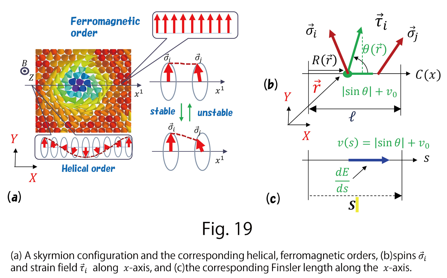
D-1. Anisotropic Deformation of Magnetic Skyrmions under Mechanical Stresses(Ref. [7])
A magnetic skyrmion is a stable spin configuration emerging in chiral magnetic materials under certain conditions. Owing to this stability, its future application to spintronics devices is expected.
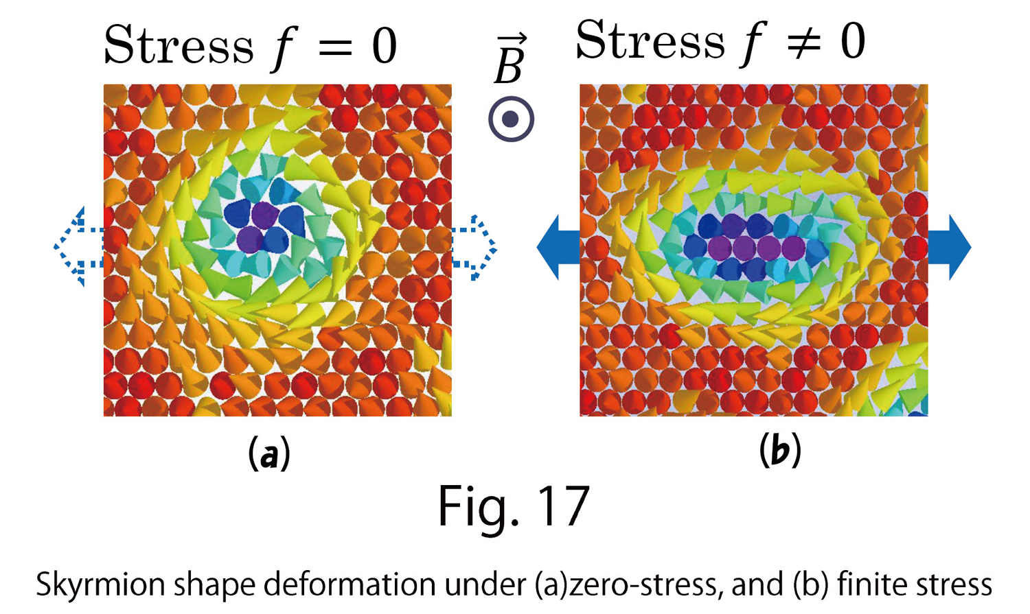
The shape of skyrmions deforms under mechanical stresses. This has been indicated theoretically and experimentally confirmed (Ref. [8]). Experimental results show that the circular skyrmion shape is oblongly deformed by tensile stresses (Fig. 17). Skyrmions represent electronic spin configurations, and therefore, it is amazing that mechanical stresses influence skyrmions.
If we consider this shape change in skyrmions to be an anisotropic deformation, we expect this deformation to be explained by the same technique as in the case of LCE. Skyrmions are considered emerging in a competition of two different interactions between spins; one is the ferromagnetic interaction (FMI) and the other is the Dzyaloshinskii-Moriya interaction (DMI). FMI and DMI, in 2-D for simplicity, are given by
(D-1)
These expressions are written using the metric tensor  in curvilinear coordinates the same as the previous expressions. In the case of Euclidean metric
  (2 x 2 unit matrix), these are
(D-2)
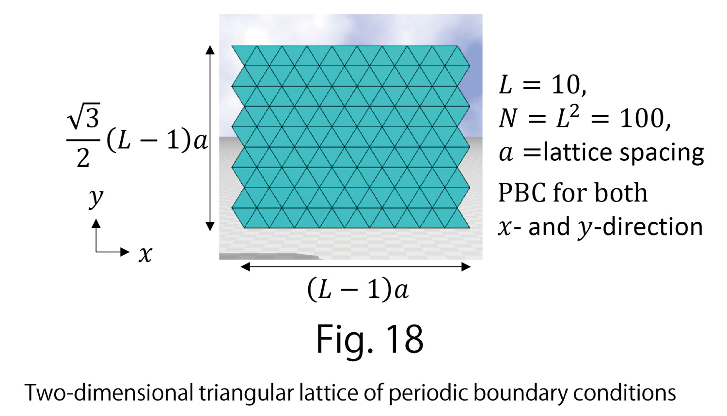
where is a unit vector denoting spin and  is its position. is variable, but is fixed. These Hamiltonians are discretized on lattices for numerical simulations. Square lattices are used in many cases; however, we use a triangular lattice (Fig. 18). The discrete Hamiltonians are as follows:
(D-3)
where is the sum of two neighboring vertices  , denotes the spin at the vertex , and
  is the unit tangential vector from the vertices to
  , The total Hamiltonian is
(D-4)
where  denote the FMI coefficient and DMI coefficient, respectively, and
  is the magnetic field.
- Ref. [7]: S.El Hog, et al. Phys. Rev. B. 104,024402 (2021) https://doi.org/10.1103/PhysRevB.104.024402
- Ref. [8]: K.Sahibata et al. Nature Nanotech. 10, 589-592(2015)
Now, to consider the problem of skyrmion shape deformation appearing on chiral magnets under mechanical tensile stress, we must answer the following questions:
- What is the internal degree of freedom responsible for the anisotropic deformation?
- Which of FMI and DMI should the Finsler metric be applied?
For (1), a position displacement is expected in atoms, and we consider a strain field  representing the direction of the displacement.
For (2), we apply the Finsler metric to DMI because an anisotropy in the DMI coefficients is indicated by Ref. [8].In Ref. [7], the Finsler metric is assumed in either FMI or DMI in the two different models, and the numerical results are presented. However, we only show the case of DMI here.
Let us consider an axis  passing through the center of a skyrmion (Fig. 19(a)). We find a so-called helical order along this axis. At the same time, we also find a ferromagnetic order between this and the neighboring skyrmion, which is not shown in Fig. 19(a). Therefore, we consider the one-dimensional integration of the axis component of
  along the axis, and its derivative (Fig. 19(b))
(D-5)
The negative sign in  is to ensure that is positive (Ref. [9]). For in the Finsler function
  we assume (Fig. 19(c))
(D-6)
In this case,  is assumed instead of
  and is a small positive number as in the previous case.
In the case of tensile stress applied along the  axis, we find that the strain becomes parallel to the axis implying that , i.e.,
  , and therefore recalling that the time distance s is defined by
  , we have
(D-7)
which will be the minimum. The line integration of this is given by
(D-8)
The fact that is small leads to an unstable helical order on the axis in Fig. 19(a). This also indicates that the DMI coefficient becomes small on this axis.
Discussions arise based on the dimensional analysis. The dimensional analysis shows that the skyrmion size becomes large (small) if the ratio of coefficients  for FMI and DMI is large (small). For this reason, since the FMI coefficient
  remains unchanged and the DMI coefficient is effectively enlarged, we find that the shape of the skyrmion becomes oblong along the axis.
- Ref. [9]: S.El Hog, et al. AirXiv http://arxiv.org/abs/2112.02173
Next, we calculate the two-dimensional metric to obtain a two-dimensional discrete Hamiltonian.
is the axis component of the metric and given by the formula
(D-9)
Thus, the two-dimensional Finsler metric is given by
(D-10)
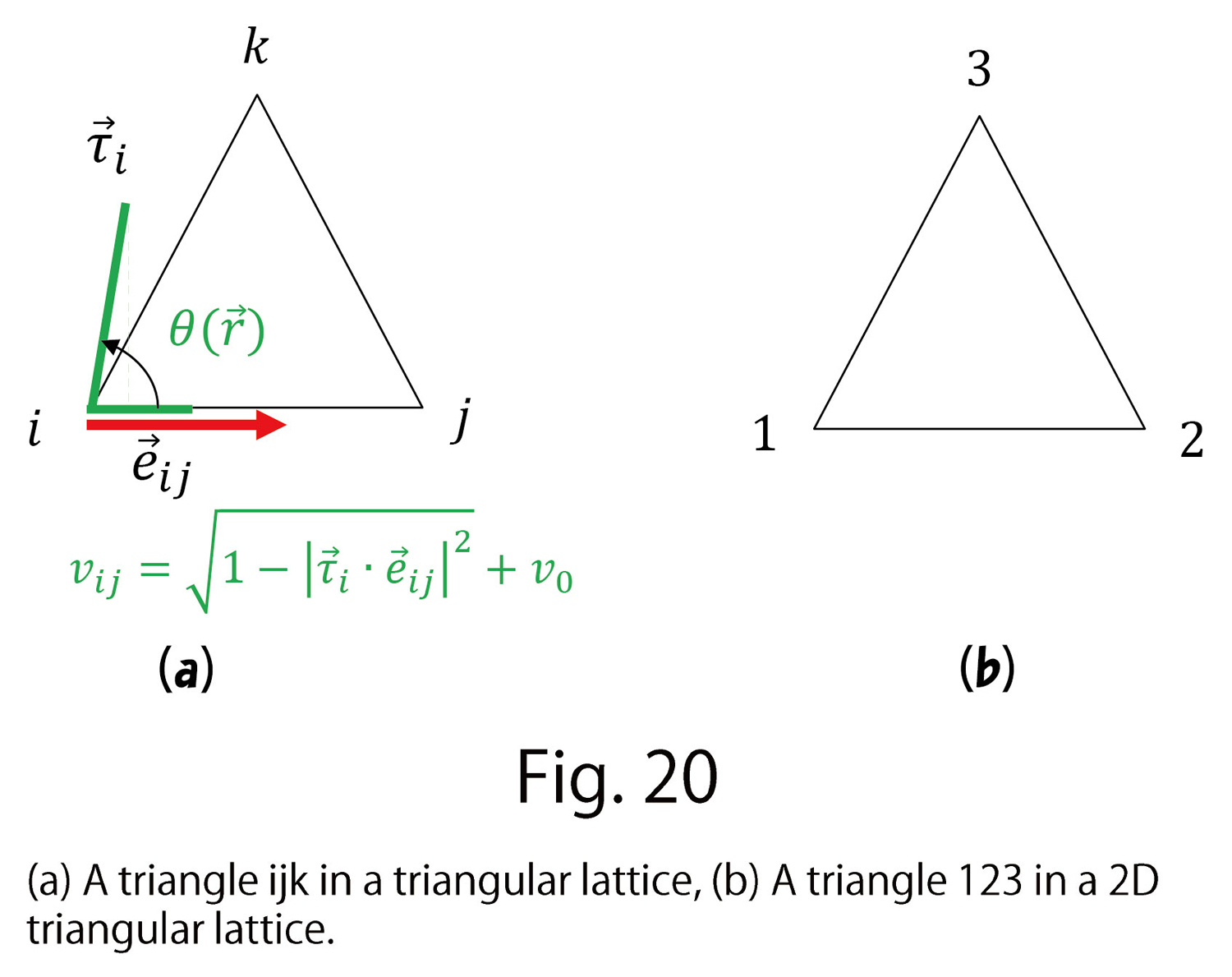
where is the inverse, is the determinant, the same as before. in is defined by using the strain  and the unit tangential vector
  such that (Fig.20(a))
(D-11)
Note that is common for both axes, however,  is different from
  because any given is different from others.
Now, we insert the obtained Finsler metric to the Hamiltonian in Eq. (D-1), which is written in the general curvilinear coordinate system. We also assume the replacements
(D-12)
where denotes the sum over triangles , For the replacement 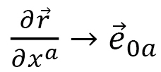 ,
,  is replaced by the unit vector. Thus, we obtain
(D-13)
We note that in the triangle 123, the coordinate origin is not always limited to vertex 1, as vertices 2 and 3 can be the origin (Fig. 20(b)). Therefore, considering the sum over the contributions from all possible coordinate origins, we perform the symmetrization procedure by replacing the indices such that 1→2, 2→3, 3→1. Including the other two different terms  and multiplying by a factor of 1/3, we have
(D-14)
which is expressed by the sum of vertices 123. By using  instead of 123, we have the expression
(D-15)
 is considered to be an effective interaction coefficient, which is defined on edge of triangle .
In the sum of triangles, appears twice for each edge ij. The other is different from the above one and slightly complex. However, the important point is that anisotropy introduced by in Eq. (D-11) is implemented in the model as an effective DMI coefficient. is originally introduced by Finsler function such that 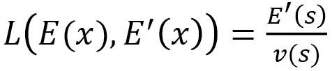 , from which the metric is originally obtained and used to discretize Hamiltonian, and the metric defined by
 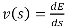 determines the scale in the time length s of Finsler. In other words, regarding the inside of materials as those governed by time length s of Finsler, we obtain the effective DMI coefficients with an anisotropy.
Next, we discuss some of the numerical results.
Figure 21(a) shows a phase diagram of magnetic field B – temperature T. Herein, three different phases, skyrmion (sky), ferromagnetic (ferro), and stripe, and their intermediate phases, skyrmion-stripe (sk-st), skyrmion-ferromagnetic (sk-fe), are specified. We find from Fig. 21(b) that skyrmions deform oblongly along the horizontal axis, to which the stress 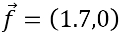 is applied. We numerically measure the horizontal and vertical lengths
  , and calculate the shape anisotropy
  by
by
(D-16)
and obtain the distribution histogram (Fig. 21(d)). Thus, the results are almost in good agreement with the reported experimental data of Ref. [8].
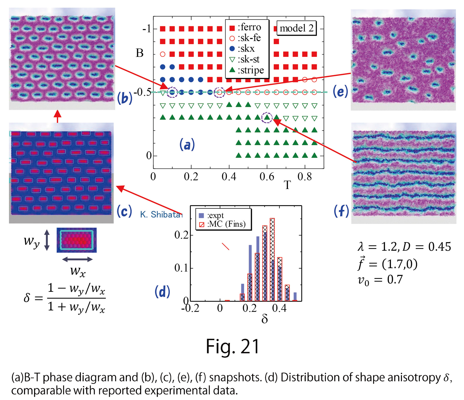
In Fig. 22(a), we plot DMI energy  per molecule in Eq. (D-15) and FMI energy
 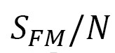 . Herein,
  is defined by
(D-17)
The two-direction arrow in Fig. 22(a) denotes the temperature region for the skyrmion phase. The absolute of decreases with increasing , and this decrement destabilizes the skyrmion. In contrast, the configurations stabilize as a ferro-magnetic order because the FMI energy decreases in the same region. This is a competition principle in two different energies, in which stabilization (destabilization) of one energy implies destabilization (stabilization) of the other.
In Fig. 22(b), we plot an anisotropy in DMI coefficient of in Eq. (D-15)
(D-18)
where  are defined by
(D-19)
The sum receives contributions from the two triangles sharing the bond , and  is the total number of bonds. We find that the anisotropy of DMI is approximately
  , implying
  . The fact that DMI is smaller in the -axis is consistent with the argument related to Eq.(D-8). We note that corresponding to the dashed line in Fig. 22(b) is the value assumed in Ref. [8] for their simulation, in which the shape deformation is predicted to be identical to the experimental result. From Fig.21(a), we have
 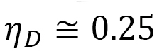 , which is relatively close to .
D-2. Deformation of Ferroelectric Polymers under Electric Field (Ref. [10])
In regard to ferroelectrics, ceramics ferroelectrics such as BaTiO3 are well-known. Ferroelectrics are a material that polarizes under an electric field and remains polarized even if the electric field is removed. For this reason, much research has been conducted from an application viewpoint.
Now, PolyVinylidene DiFluoride (PVDF) is ferroelectric material, and it is a polymer. The study in Ref. [11] by H.Kawai is well-known. A special observation is that strains by electric field are relatively larger than those in ceramics ferroelectrics. For this reason, it attracts attention from the viewpoint of application to actuators.
Since PVDF is a polymer, and the Hamiltonian is basically the same as that of LCE, there is a Gaussian bond potential. The only difference from LCE is the internal degree of freedom (IDF) that causes anisotropy. The IDF in PVDF is a polarization vector of dielectrics. The polarization vector has polarity. Hence, an essential difference between PVDF and LCE is whether the IDF is polar or non-polar.
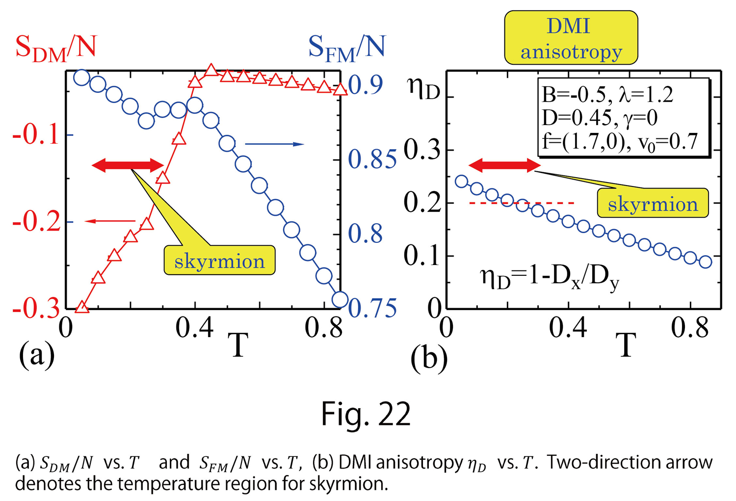
In the numerical simulations, we use 3D lattice in Fig. 23(a), calculate strains and the polarization along -axis, and compare them with reported experimental data. The 3D disk is discretized by tetrahedrons in Fig. 23(b), and this is also the same as for LCE.
Anisotropy is defined by
(D-20)
This is the same as the case for skyrmions, because the angle is between the polarization vector and the coordinate axis. The 3D Hamiltonian is also the same as that in LCE, and the expression is
(D-21)
where , denote the sum over bonds and the sum over tetrahedrons sharing the bond , and is defined on the bond in the tetrahedron  in Fig.12(b). This can also be written by using the sum over tetrahedrons and the sum over bonds of the tetrahedron such that
(D-22)
- Ref. [10] V.Egorov et al.Phys. Lett. A 396 (2021) 127230 https://doi.org/10.1016/j.physleta.2021.127230
- Ref. [11] H. Kawai, The Piezoelectricity of Polyvynilidene Fluoride, Jpn. J. Appl. Phys. Vol.8, p.975 (1969).
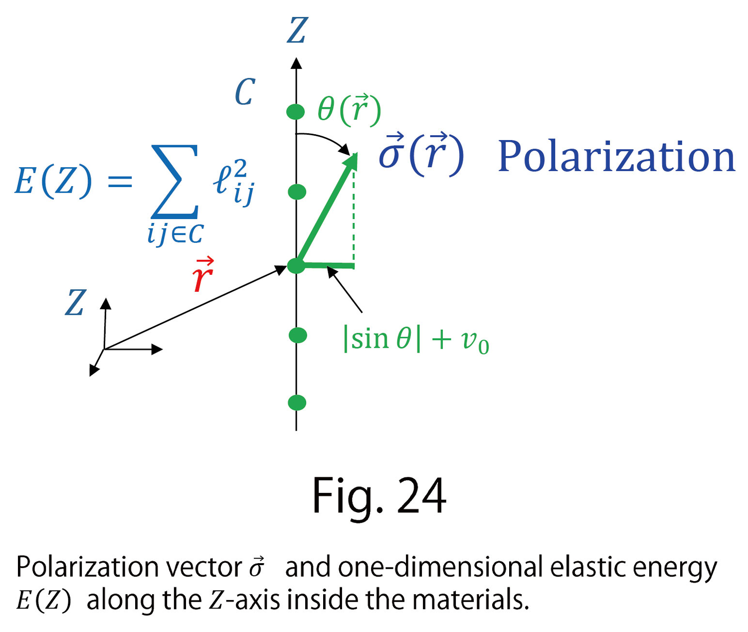
Here, we show the reason why PVDF shrinks under an electric field. For this purpose, we consider a one-dimensional integral of the bond potential along the Z-axis parallel to the electric field such that (Fig. 24)
(D-23)
This is the same as in the case of LCE.
For
From the one-dimensional energy 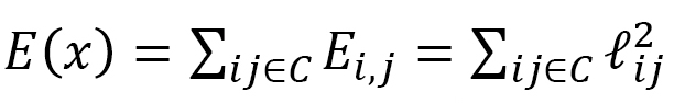 and
and 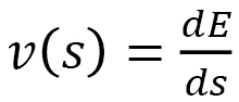 , we have
 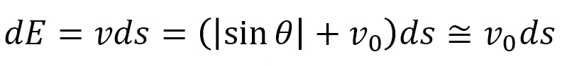 , Hence, by the integration, we obtain
 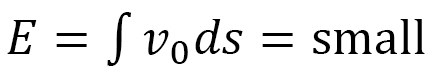 , where is also assumed to be a small positive number. Since the left-hand side is
 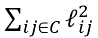 , we finally obtain
 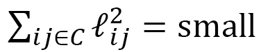 . This implies that molecular distance becomes small along the electric field direction. Moreover, recalling that elastic energy includes a tension coefficient and that the elastic energy is constant, we find that the tension coefficient effectively increases along the Z-axis because decreases. Namely, the fact that the tension coefficient increases while the electric field is applied shares the same principle as the case of LCE, although it is the converse.
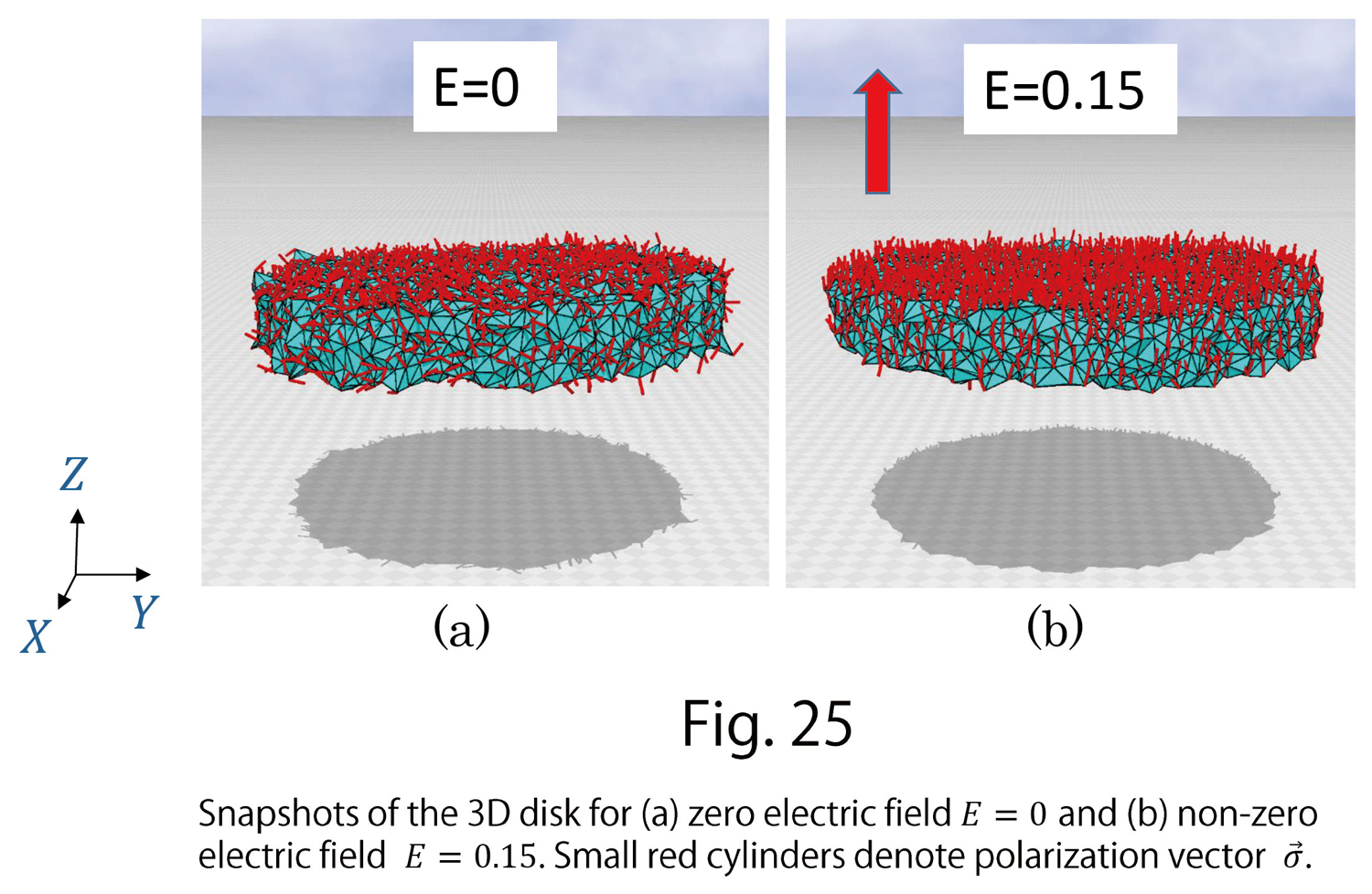
Snapshots of the simulation results are shown in Figs. 25(a),(b), where (a) and (b) are configurations of zero (non-zero) electric field, and small red cylinders represent the polarization vector The reason why is not entirely random is because PVDF is a ferroelectric and has non-zero polarization even for zero electric fields. In this case, the non-zero polarization aligns to Z-axis the same as the electric field direction.
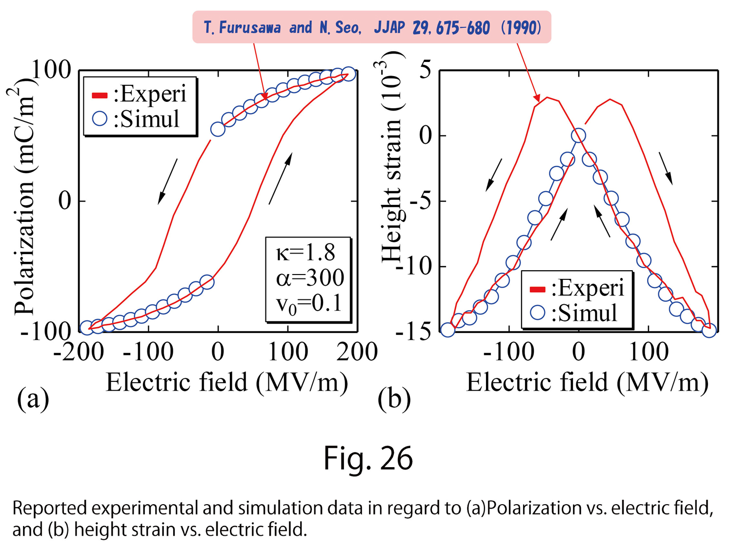
Figures 26(a),(b) show reported experimental data in Ref. [12] and the simulation results of the Finsler geometry model; polarization vs. electric field in Fig.26(a), and the strain vs. electric field in Fig. 26(b). Here the details of units assumed in the simulations are skipped; however, the strain is dimensionless and must not be modified. The strains are the same as those of the lattice deformation. These two sets of simulation data are obtained with the same set of parameters. Moreover, anisotropy in the interaction coefficient is dynamically generated by the electric field. These indicate that the results of the Finsler geometry model are precisely identical with experimental data.
Acknowledgments
H. Koibuchi acknowledges Dr. Hiroshi Fukumura, the former president of Sendai College of Technology, for a chance and environment to continue research activity during the period of reemployment. He acknowledges all authors in the joint research. He also acknowledges Dr. Takashi Matsuhisa, Dr. Madoka Nakayama, and Dr. Kohei Tasaki for helpful discussions. This home page is supported in part by JSPS Grant-in-Aid for Scientific Research on Innovative Areas "Discrete Geometric Analysis for Materials Design": Grant Number 20H04647.
- Ref. [12] T.Furusawa and N.Seo,Electristriction as the origin of Piezoelectricity in Ferroelectric Polymers, JJAP 29,675-680 (1990).